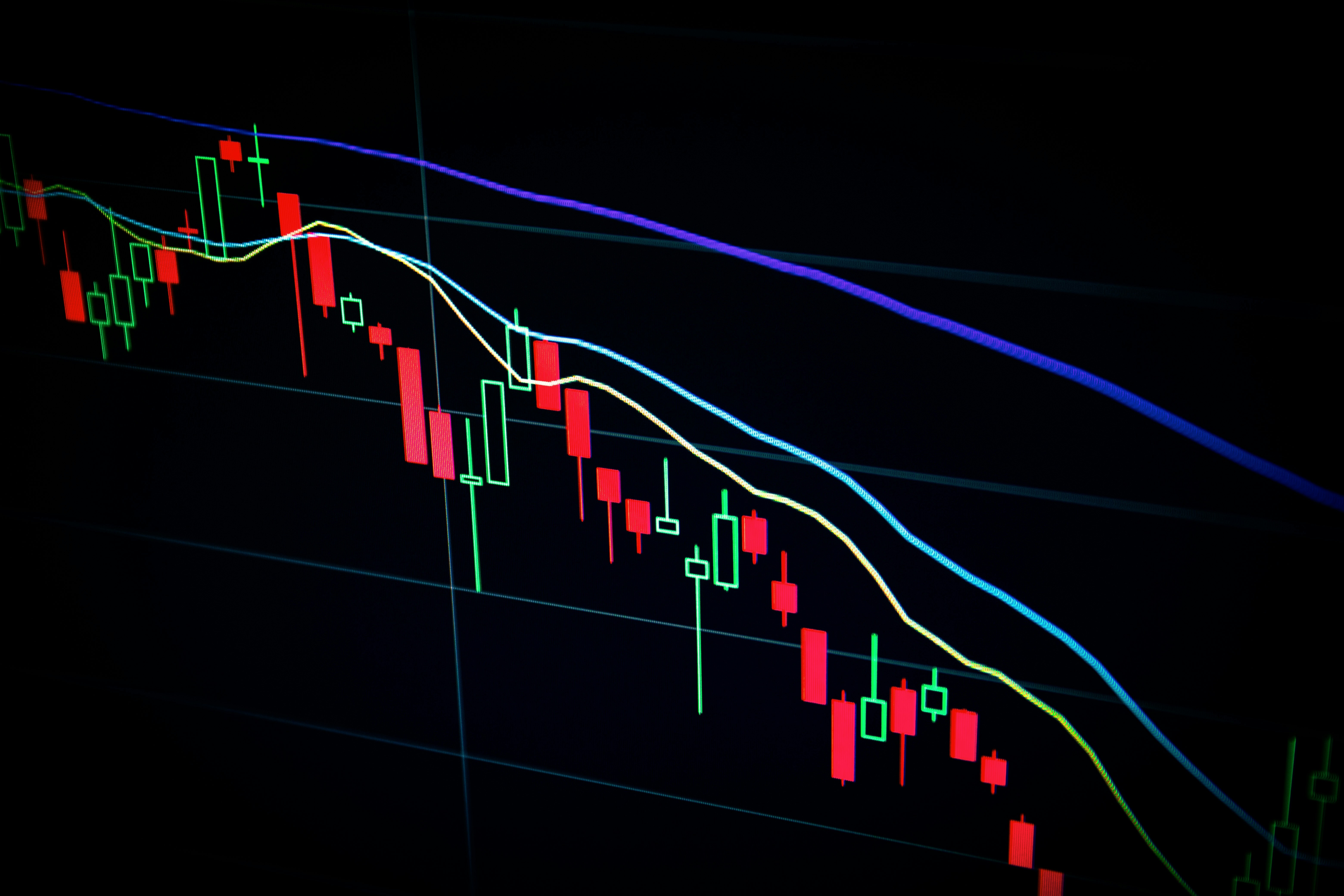
Getting Started with Quantitative Trading

Quantitative trading combines mathematical models, statistical analysis, and programming to make trading decisions. In this post, I'll guide you through the essential components of building a quantitative trading system.

The Foundation: Data Collection

The first step in any quantitative trading system is gathering high-quality data. This includes:

• Market data (prices, volumes, order books)
• Fundamental data (financial statements, economic indicators)
• Alternative data (news sentiment, social media trends)

import yfinance as yf
import pandas as pd

# Fetch historical data
def fetch_market_data(symbol, start_date, end_date):
    ticker = yf.Ticker(symbol)
    data = ticker.history(start=start_date, end=end_date)
    return data

# Example usage
spy_data = fetch_market_data("SPY", "2023-01-01", "2024-03-20")

Feature Engineering

Once you have the data, the next step is to create meaningful features that can predict future price movements. Common features include:

1. Technical indicators (RSI, MACD, Bollinger Bands)
2. Price momentum
3. Volatility measures
4. Market regime indicators

Here's an example of calculating the Relative Strength Index (RSI):

def calculate_rsi(data, period=14):
    delta = data['Close'].diff()
    gain = (delta.where(delta > 0, 0)).rolling(window=period).mean()
    loss = (-delta.where(delta < 0, 0)).rolling(window=period).mean()
    rs = gain / loss
    return 100 - (100 / (1 + rs))

Strategy Development

The core of quantitative trading is the strategy. A good strategy should:

• Have a clear hypothesis
• Be based on sound economic principles
• Include proper risk management
• Be thoroughly backtested

Here's a simple mean reversion strategy:

def mean_reversion_strategy(data, window=20, std_dev=2):
    # Calculate rolling mean and standard deviation
    rolling_mean = data['Close'].rolling(window=window).mean()
    rolling_std = data['Close'].rolling(window=window).std()
    
    # Generate signals
    upper_band = rolling_mean + (rolling_std * std_dev)
    lower_band = rolling_mean - (rolling_std * std_dev)
    
    # Long when price is below lower band, short when above upper band
    signals = pd.Series(0, index=data.index)
    signals[data['Close'] < lower_band] = 1
    signals[data['Close'] > upper_band] = -1
    
    return signals

Backtesting

Before deploying any strategy, it's crucial to test it on historical data. A good backtest should:

1. Account for transaction costs
2. Consider market impact
3. Include proper position sizing
4. Test across different market regimes

Risk Management

No strategy is complete without proper risk management. Key considerations include:

• Position sizing
• Stop-loss levels
• Portfolio diversification
• Drawdown limits

Next Steps

This is just the beginning of your quantitative trading journey. As you progress, you'll want to explore:

1. Machine learning models for prediction
2. High-frequency trading strategies
3. Portfolio optimization techniques
4. Real-time data processing

Remember that successful quantitative trading requires continuous learning and adaptation. The market is always evolving, and so should your strategies.

Resources

• QuantConnect - Platform for strategy development
• Quantopian - Educational resources
• TradingView - Charting and analysis tools
• Investopedia - Educational content

Stay tuned for more posts about specific aspects of quantitative trading!